Impedance and Admittance Control for Robotic Arms
Abstract
This project explores the mathematical foundations and implementations of impedance and admittance control schemes for robotic manipulators. These complementary approaches enable robots to interact safely and effectively with their environment by regulating the dynamic relationship between forces and positions. The mathematical models and implementations presented here provide insights into how these control strategies create compliant robotic behavior while maintaining position accuracy, essential for safe human-robot interaction and delicate manipulation tasks.
Mathematical Foundation: Impedance and Admittance Control
Impedance and admittance control are complementary approaches to robot force control, each with distinct mathematical foundations and practical implementations:
Mechanical Impedance Principle
Mechanical impedance defines the dynamic relationship between force and motion:
F = Z(s) · X(s)
Where F is force, X is position, and Z(s) is the impedance transfer function in the Laplace domain, typically modeled as a mass-spring-damper system:
Z(s) = Ms² + Bs + K
- M: Virtual inertia (mass) parameter
- B: Virtual damping parameter
- K: Virtual stiffness parameter
- These parameters define the robot's dynamic behavior when interacting with the environment
Impedance vs. Admittance Control
Admittance is the mathematical inverse of impedance, defining position response to applied force:
X(s) = Y(s) · F(s) = Z⁻¹(s) · F(s)
Where Y(s) is the admittance transfer function:
Y(s) = 1/(Ms² + Bs + K)
- Impedance control: Force output from motion error (ideal for robots with good backdrivability)
- Admittance control: Motion command from force error (ideal for stiff, high-geared robots)
- Both achieve compliant behavior but with different control structures
Impedance Control Mathematical Model
The classical impedance control law in task space coordinates:
M(ẍ - ẍd) + B(ẋ - ẋd) + K(x - xd) = Fext
Which leads to the joint-space torque command:
τ = JT(q)[Fd - M(ẍ - ẍd) - B(ẋ - ẋd) - K(x - xd)]
- J(q): Jacobian matrix mapping joint velocities to end-effector velocities
- xd, ẋd, ẍd: Desired position, velocity, and acceleration
- Fext: External force measured at the end-effector
- Fd: Desired force (often zero for pure motion control)
Admittance Control Mathematical Model
The admittance control generates a modified trajectory based on measured external forces:
M(ẍ - ẍr) + B(ẋ - ẋr) + K(x - xr) = Fext - Fd
Where the reference trajectory xr is followed by an inner position control loop:
qd = IK(xr)
- xr, ẋr, ẍr: Reference position, velocity, and acceleration
- IK(): Inverse kinematics function
- Fext: Measured external force
- qd: Desired joint positions sent to the robot's position controller
Robot behaves like a mass-spring-damper system, generating forces in response to position deviations
Robot modifies its position trajectory in response to measured external forces
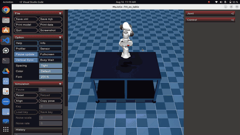
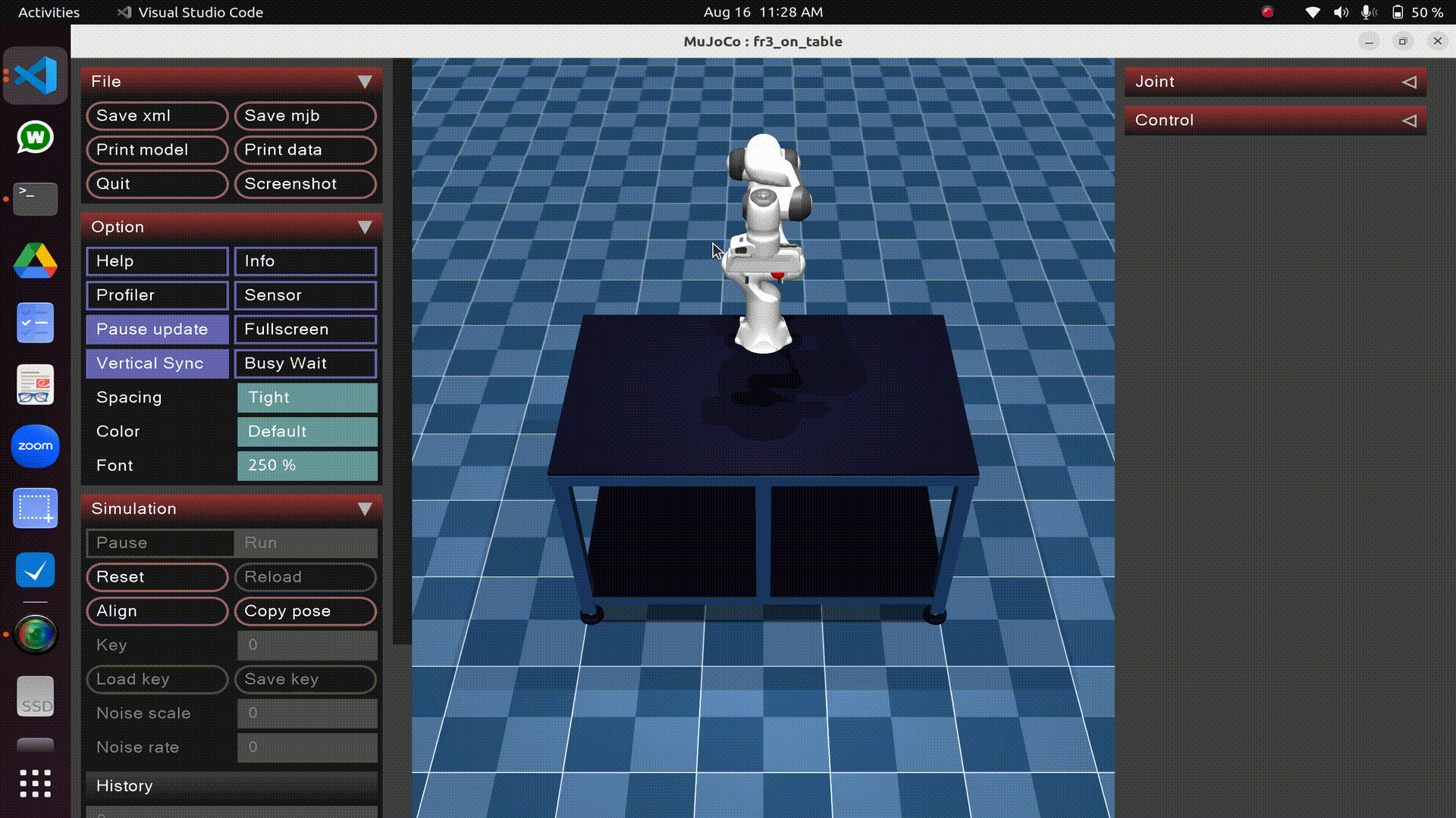
Control Scheme Comparison
The two GIFs above demonstrate the complementary nature of impedance and admittance control schemes:
Impedance Control Characteristics
Impedance control exhibits these key behaviors:
- Directly commands joint torques based on measured position errors
- Better suited for robots with good backdrivability and accurate torque control
- Typically uses lower control loop frequencies (1-5 kHz) due to direct torque commands
- Provides more responsive interaction but may have position tracking errors
- Control flow: Position error → Force command
Admittance Control Characteristics
Admittance control demonstrates these distinctive properties:
- Uses measured external forces to modify position trajectories
- Better suited for high-geared robots with good position control but poor torque control
- Often requires force/torque sensors for accurate interaction force measurement
- Typically uses higher control loop frequencies for stable operation
- Control flow: Force measurement → Position modification
Key Theoretical Concepts
Mechanical Duality
Impedance and admittance control form a dual relationship in control theory, representing inverse approaches to the same interaction problem
Parameter Tuning
Virtual mass, damping, and stiffness parameters directly influence robot behavior, with higher stiffness providing better position tracking but reduced compliance
Contact Stability
Both control schemes must be carefully tuned to maintain stability during environmental contact, with damping being critical for preventing oscillations
Hardware Considerations
The choice between impedance and admittance control is often determined by robot hardware capabilities, particularly joint backdrivability and sensing
Implementation Details
The implementation of impedance and admittance control follows these key algorithmic steps:
Impedance Control Algorithm
1. Read current joint positions q and velocities q̇
2. Compute forward kinematics and Jacobian: x = FK(q), J = J(q)
3. Measure external force Fext (using F/T sensor or observer)
4. Compute the impedance model forces:
Fimp = M(ẍd - ẍ) + B(ẋd - ẋ) + K(xd - x)
5. Transform to joint torques and command actuators:
τcmd = JT(Fimp + Fext)
Admittance Control Algorithm
1. Measure external force Fext using force/torque sensor
2. Compute reference trajectory modification using admittance model:
M(ẍr - ẍd) + B(ẋr - ẋd) + K(xr - xd) = Fext
3. Numerically integrate to get modified reference trajectory xr
4. Compute inverse kinematics to get joint positions:
qr = IK(xr)
5. Send qr to the robot's position controller
Implementation Considerations
- Real-time requirements: Impedance control typically needs 1-5 kHz loop rate
- Proper noise filtering of force/torque measurements to avoid instability
- Velocity estimation from position measurements (if necessary)
- Safety measures including virtual walls and force/velocity limits
- Gradual parameter adjustment during contact transitions to avoid jerky motions
Applications and Performance Comparison
Impedance and admittance control have distinct application domains and performance characteristics:
Industrial Applications
Admittance control excels in precise assembly tasks with stiff robots, while impedance control is preferred for delicate handling operations
Human-Robot Interaction
Both schemes enable safe physical interaction, with adjustable compliance parameters directly affecting perceived robot behavior
Manipulation Tasks
Surface-following, peg-in-hole insertion, and cooperative tasks all benefit from force-based control with appropriately tuned stiffness
Technical Considerations
- Stability analysis using Lyapunov methods ensures safe operation across various environments
- Time delay compensation is essential, especially for admittance control
- Friction and gravity compensation improve performance in both control schemes
- Singularity handling is required when operating near kinematic limits
- Variable impedance/admittance parameters can adapt to changing tasks
Advanced Extensions
- Task-oriented impedance control with coordinate frame selection
- Learning-based parameter tuning from human demonstrations
- Hybrid force/position control for constrained manipulation
- Multi-arm cooperative control with internal force regulation
- Energy-based passivity control for guaranteed stability
Conclusion
This project examines the mathematical foundations and implementations of impedance and admittance control for robotic manipulators. Both approaches provide elegant solutions to the fundamental challenge of controlling robot-environment interactions by establishing dynamic relationships between forces and positions. The mass-spring-damper model provides an intuitive framework that translates into effective control algorithms with tunable parameters directly influencing robot behavior.
The choice between impedance and admittance control largely depends on robot hardware characteristics, with impedance control being ideal for robots with good backdrivability and torque control, while admittance control excels for high-geared, stiff robots with precise position control. Both schemes find extensive applications in industrial robotics, human-robot interaction, and delicate manipulation tasks. The mathematical models presented here provide a strong foundation for understanding and implementing these complementary control strategies, enabling safe and effective robotic interaction with dynamic environments.